Things could not look more grim for BlackBerry right now....They are losing market-share at an alarming rate, and they have not produced a phone or OS with any sort of WOW factor as of late. Management is a laughing stock in the sense that they have two CEO's (Seriously guys?), what else could go wrong? That depends on what is next....
What is next? I will give my opinions on the subject, then open it for comments from abroad.
Without any major innovations apparent on the horizon, RIMM 's price will continue to get hammered by traders and institutional investors alike. Why? On top of the aforementioned market share decline issue, they no longer have any sort of competitive advantage over AAPL or GOOG in the smart phone OS industry. Their once claim to fame was the Enterprise system exclusivity which is now a thing of the past. So, while RIMM's price continues to decline what could happen?
1. Will they be forced to buy-back their shares and pull themselves off the market?
2. Will they be purchased by a private-equity firm or even someone like MSFT ??
3. Will they innovate and surprise us with a new and exciting product (on their own...)?
My current vote goes to... 2. I believe that Microsoft will buy BlackBerry and finally put their hat in the smart phone arena (for real this time)!
Lets hear what you have to say!
Monday, June 20, 2011


Friday, June 17, 2011
Thoughts on an APPL 10-1 Split?
We will shift gears for a little while here while I build code for the next topic of "Option Volatility" and discuss a topic that is on a lot of traders minds...
AAPL needs to conduct a 10-1 split.....
I know this is a practice that is highly debated, so I wanted to spark some discussion here about the merits and drawbacks associated with such a move.
I found an interesting article AAPL P/E Ratio. Basically, Apple trades at a relatively low P/E ratio (~15 P/E) when compared to current growth companies like AMZN (~80 P/E) and NFLX (~70.58). Why??? AAPL consistently tops estimates and over performs on all metrics, while AMZN and NFLX rarely beat expectations.
My opinion : AAPL is the MOST EXPENSIVE and CHEAP stock all at the same time.
It is CHEAP from almost every valuation metric (AAPL's PEG value is currently <1.... ~0.98), BUT.... it is EXPENSIVE in the sense that there is only a small market of individual investors who are willing to spend $330 dollars to get 1 share...
So how does AAPL save their distressed P/E ratio??
A 10-1 split, I would be willing to bet substantial amounts of money that if AAPL conducted a 10-1 split and moved the share price down to $33 dollars a share, that within 1 year it would be trading over $100 dollars a share....
What is their to lose?? That is where you come in.... Lets get a healthy debate going here.
AAPL needs to conduct a 10-1 split.....
I know this is a practice that is highly debated, so I wanted to spark some discussion here about the merits and drawbacks associated with such a move.
I found an interesting article AAPL P/E Ratio. Basically, Apple trades at a relatively low P/E ratio (~15 P/E) when compared to current growth companies like AMZN (~80 P/E) and NFLX (~70.58). Why??? AAPL consistently tops estimates and over performs on all metrics, while AMZN and NFLX rarely beat expectations.
My opinion : AAPL is the MOST EXPENSIVE and CHEAP stock all at the same time.
It is CHEAP from almost every valuation metric (AAPL's PEG value is currently <1.... ~0.98), BUT.... it is EXPENSIVE in the sense that there is only a small market of individual investors who are willing to spend $330 dollars to get 1 share...
So how does AAPL save their distressed P/E ratio??
A 10-1 split, I would be willing to bet substantial amounts of money that if AAPL conducted a 10-1 split and moved the share price down to $33 dollars a share, that within 1 year it would be trading over $100 dollars a share....
What is their to lose?? That is where you come in.... Lets get a healthy debate going here.
Thursday, June 16, 2011
Final Part of Pair Trading Analysis Using Python 3.1!
Before I begin, here are the links to the source code itself (pairAnalysis.py) and two examples of data for closing prices of Coke and Pepsi.
Here is the source code in Python: (Make sure to open it with the Pythone IDLE)
pairAnalysis.py
Also, it is worth noting that every time you wish to conduct an analysis you must close out the GUI and Python terminal and re- run it to prevent overlapping data structures.
Here are the files containing the closing prices for Coke and Pepsi over the last three years:
KO.txt
PEP.txt
Download these three files and save them to a directory you can remember because through the GUI created by the source code you will select the files for analysis.
So after downloading the source code and then opening the file with Python IDLE, you are now reading to run the program. You can do this simply by pressing F5.
You should now be looking at a GUI (Graphical User Interface) that looks like this:
 1. Click the top Select File button and select the KO.txt file that you downloaded. Do the same for the
Stock 2 but select the PEP.txt file.
2. Enter the current price of KO in the Current Price of Stock 1 box, and enter the current price of PEP in the box below.
3. Select the number of data points you wish to analyze.
4. Set the variance increment, this is the range plus/minus the average difference that points must fall in.
5. Set the threshold percentage, this is the necessary percentage of data points that must fall within the average difference plus/minus the variance you set in the box below.
You should now be looking at something like this:
 We are now ready to press the Compute Results button. After pressing the compute results button we will be looking at this screen:
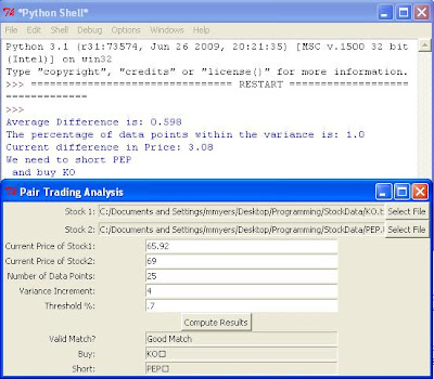 Notice first off that it rendered a "Good Match" decision. Above the GUI, I included the terminal for Python with some observations that were made while going through the code. It states that the average difference in daily price is 0.598, which means that on average Pepsi closes 60 cents higher than Coke does (Because the difference is calculated as Stock2 - Stock1). The next thing we see is that 100 percent of the data points fell within the variance we set of 4. This means that 100% of the difference data points (difference in daily closing price for each of the last 25 days) fell within the range of
[0.598 - 4 , 0.598 + 4] or [-3.402 , 4.598]. Now, with a 100% result, we surpass the threshold we set of 0.7 or 70%. That is why we have a "Good Match" decision and continue on to calculate adjusted prices. After calculating adjusted prices we see that KO is undervalued and PEP is overvalued. We calculate the adjusted prices in this case by adding the average difference to the current price of
KO (65.92 + 0.598 = 66.518) and subtracting the average difference from the current price of
PEP (69 - 0.598 = 68.402). Because 66.518 (adjusted price of Coke) is less than 68.402 (adjusted price of Pepsi), we say buy Coke and short Pepsi.
Going forward..... Download as many different securities as you have time for and start conducting analysis on them! See if you find any stocks that trade in pairs that you might not expect, BECAUSE if you do not expect them to be pairs - then most people do not either. This means they are ripe for profit opportunities!! I encourage you to think outside the box, try things like comparing OIL index prices with different shipping companies or Cotton indexes with different clothing companies. Keep in mind that the tighter you set the variance and the higher you set the threshold, the more accurate the decision is. For instance, if you set a variance of 1 and a threshold of 95%, then if you get a "Good Match" indicator you can conclude strongly that they trade in a tight pair pattern.
Please leave comments if you have questions or find any interesting results!
Have a great day!
Here is the source code in Python: (Make sure to open it with the Pythone IDLE)
pairAnalysis.py
Also, it is worth noting that every time you wish to conduct an analysis you must close out the GUI and Python terminal and re- run it to prevent overlapping data structures.
Here are the files containing the closing prices for Coke and Pepsi over the last three years:
KO.txt
PEP.txt
Download these three files and save them to a directory you can remember because through the GUI created by the source code you will select the files for analysis.
So after downloading the source code and then opening the file with Python IDLE, you are now reading to run the program. You can do this simply by pressing F5.
You should now be looking at a GUI (Graphical User Interface) that looks like this:

Stock 2 but select the PEP.txt file.
2. Enter the current price of KO in the Current Price of Stock 1 box, and enter the current price of PEP in the box below.
3. Select the number of data points you wish to analyze.
4. Set the variance increment, this is the range plus/minus the average difference that points must fall in.
5. Set the threshold percentage, this is the necessary percentage of data points that must fall within the average difference plus/minus the variance you set in the box below.
You should now be looking at something like this:

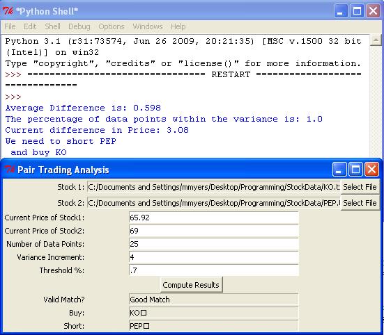
[0.598 - 4 , 0.598 + 4] or [-3.402 , 4.598]. Now, with a 100% result, we surpass the threshold we set of 0.7 or 70%. That is why we have a "Good Match" decision and continue on to calculate adjusted prices. After calculating adjusted prices we see that KO is undervalued and PEP is overvalued. We calculate the adjusted prices in this case by adding the average difference to the current price of
KO (65.92 + 0.598 = 66.518) and subtracting the average difference from the current price of
PEP (69 - 0.598 = 68.402). Because 66.518 (adjusted price of Coke) is less than 68.402 (adjusted price of Pepsi), we say buy Coke and short Pepsi.
Going forward..... Download as many different securities as you have time for and start conducting analysis on them! See if you find any stocks that trade in pairs that you might not expect, BECAUSE if you do not expect them to be pairs - then most people do not either. This means they are ripe for profit opportunities!! I encourage you to think outside the box, try things like comparing OIL index prices with different shipping companies or Cotton indexes with different clothing companies. Keep in mind that the tighter you set the variance and the higher you set the threshold, the more accurate the decision is. For instance, if you set a variance of 1 and a threshold of 95%, then if you get a "Good Match" indicator you can conclude strongly that they trade in a tight pair pattern.
Please leave comments if you have questions or find any interesting results!
Have a great day!
Wednesday, June 15, 2011
Part Two of Pair Trading Using Python 3.1!!
Today I am going to showcase the methodology, from a coding stand-point, we would use to determine whether two securities are good candidates for pair trading. Whereas, the next posting will show the actual source code that I wrote to do the analysis.
Step 1: We need to get the data. The analysis is worthless without having sufficient data to use. For this exercise, I pulled 3 years worth of daily closing prices from AAPL Closing Prices . Notice, this data source is freely available and located at Yahoo! Finance . Make sure you set the parameters at the top to indicate that you want daily prices, and make sure you select the same time frame for each set of data you want to compare. In this example, I pulled Jan 1, 2008 to yesterday (Jun 14, 2011). After we arrive at this web address, at the bottom of the page is a link to "Download to Spreadsheet." Select this link and now the data should be in a spreadsheet. Next, we open a blank ".txt" file and type in the Ticker Symbol for the Security you just pull data from on the top line of the file, e.g. "AAPL". Lastly, we copy the closing price column from the spreadsheet we just downloaded and paste it into the .txt file below the ticker symbol.
Step 2: After you have pulled one data set, repeat the same procedures outlined in Step 1 for the security you wish to compare with the first data set. MAKE SURE YOU SELECT THE SAME TIME FRAME! We should now have two .txt files titled with the two ticker symbols you wish to compare, for example, KO.txt and PEP.txt.
Step 3: Now that we have two data sets that represent the closing prices of two securities for a set period of time, we are ready to do some analysis. The first step in analysis is to calculate an average difference in price for the two securities during the time frame. For example, if we select a time frame of the last 50 closing prices, we want to know the difference in closing price between the two securities for every day in that 50 day window. We will store those "difference data points" in a list. Then we will calculate the average difference by taking the average of the "difference data points list." This overall average difference is going to be critical in determining whether or not the two securities represent a "good" pair.
Step 4: The next step in the analysis is to determine how many of those "difference data points" are "close" to the actual average difference. In other words, we are checking to see if the average resulted from consistent differences in price, or from wild, varying differences. This is important to know because in order to profit from price movement, we want there to be a consistent difference in price. That way, when the prices move away from this average difference, we can make "bets" on the fact that they will once again return to that average difference in price. The way we will approach this problem is by setting a "variance." We want to check how many of the "difference data points" in the list fall within the range of the "average difference" plus/minus a "variance." This will result in a simple "count" of the number of data points in the "difference data points list" that fall within the overall average difference plus/minus a variance that we set earlier.
Step 5: Now that we have this "count" value from Step 4, we will now do some more analysis to determine if that is a sufficiently large count value. Simply, we set an overall "threshold percentage" that represents the percentage of data points that need to fall within the variance range to represent a "good" pair. If the "count" value divided by the total number of data points we selected is greater than the "threshold percentage" that we established, then we say that the two securities are a "Good Match."
Step 6: Lastly, if the two securities resulted in a "Good Match" decision, then we need to do some analysis to determine which security needs to be shorted and which one needs to be bought. If the decision rendered was that they were a "Bad Match", then the analysis is done and we do nothing with that pair. In the case of a "Good Match", the logic to determine which one is a short and a buy is relatively simple. First, it is noteworthy that we are calculating the difference in data points as Security2 closing price - Security1 closing price. In other words, the first security you get data from is being subtracted from the second security you gathered data on. So, if the overall average difference is greater than or equal to 0, then that means that on average Security2's price is greater than Security1's price. With this information we are ready to create adjusted prices. If the average difference in price is greater than or equal to 0, then the adjusted price for Security1 is equal to the current price of Security1 plus the average difference between the two securities. The adjusted price for Security2 would then equal the current price of Security2 minus the average difference between the two securities. In the case that the average difference is less than or equal to 0 (meaning on average the price of Security1 is greater than Security2), we do the opposite and subtract the average difference from the current price of Security1 and add the average difference to the current price of Security2 to come up with the overall adjusted prices. Finally, if the adjusted price of Security1 is greater than Security2, that would mean that we should short Security1 and buy Security2. If the adjusted price of Security2 is greater than Security1, then we would short Security2 and buy Security1.
Summarily, we are getting the data points for two different securities. We are making a list of the difference in prices for each day. We then take the average of that list of differences. We are then calculating a percentage based on how many of those data points are close to the average difference. If the percentage is high, we would say the two securities are a good match because that means that the difference in price is usually the same between the two securities. Last, we do some math to see which one is priced too high, and we short that security and buy the other one.
Hopefully, this explanation of the methodology is sufficient for you understanding. However, if you still do not fully understand, then the next posting containing the source code should drive the point across. Do keep in mind that my Inbox is always open for questions ( progamtotrade@gmail.com ).
A preview of the agenda for upcoming posts:
Next Post: Source code for pair trading analysis
Next Series: How does the delta value for an option as well as the corresponding option premium relate to the premium of a VIX (Volatility Index) option for the same time frame? Is there a relationship? If so, what is the underlying relationship and how can it be utilized for profits?? We will explore these questions through the use of functional programming in Python 3.1!
Take Care!
Step 1: We need to get the data. The analysis is worthless without having sufficient data to use. For this exercise, I pulled 3 years worth of daily closing prices from AAPL Closing Prices . Notice, this data source is freely available and located at Yahoo! Finance . Make sure you set the parameters at the top to indicate that you want daily prices, and make sure you select the same time frame for each set of data you want to compare. In this example, I pulled Jan 1, 2008 to yesterday (Jun 14, 2011). After we arrive at this web address, at the bottom of the page is a link to "Download to Spreadsheet." Select this link and now the data should be in a spreadsheet. Next, we open a blank ".txt" file and type in the Ticker Symbol for the Security you just pull data from on the top line of the file, e.g. "AAPL". Lastly, we copy the closing price column from the spreadsheet we just downloaded and paste it into the .txt file below the ticker symbol.
Step 2: After you have pulled one data set, repeat the same procedures outlined in Step 1 for the security you wish to compare with the first data set. MAKE SURE YOU SELECT THE SAME TIME FRAME! We should now have two .txt files titled with the two ticker symbols you wish to compare, for example, KO.txt and PEP.txt.
Step 3: Now that we have two data sets that represent the closing prices of two securities for a set period of time, we are ready to do some analysis. The first step in analysis is to calculate an average difference in price for the two securities during the time frame. For example, if we select a time frame of the last 50 closing prices, we want to know the difference in closing price between the two securities for every day in that 50 day window. We will store those "difference data points" in a list. Then we will calculate the average difference by taking the average of the "difference data points list." This overall average difference is going to be critical in determining whether or not the two securities represent a "good" pair.
Step 4: The next step in the analysis is to determine how many of those "difference data points" are "close" to the actual average difference. In other words, we are checking to see if the average resulted from consistent differences in price, or from wild, varying differences. This is important to know because in order to profit from price movement, we want there to be a consistent difference in price. That way, when the prices move away from this average difference, we can make "bets" on the fact that they will once again return to that average difference in price. The way we will approach this problem is by setting a "variance." We want to check how many of the "difference data points" in the list fall within the range of the "average difference" plus/minus a "variance." This will result in a simple "count" of the number of data points in the "difference data points list" that fall within the overall average difference plus/minus a variance that we set earlier.
Step 5: Now that we have this "count" value from Step 4, we will now do some more analysis to determine if that is a sufficiently large count value. Simply, we set an overall "threshold percentage" that represents the percentage of data points that need to fall within the variance range to represent a "good" pair. If the "count" value divided by the total number of data points we selected is greater than the "threshold percentage" that we established, then we say that the two securities are a "Good Match."
Step 6: Lastly, if the two securities resulted in a "Good Match" decision, then we need to do some analysis to determine which security needs to be shorted and which one needs to be bought. If the decision rendered was that they were a "Bad Match", then the analysis is done and we do nothing with that pair. In the case of a "Good Match", the logic to determine which one is a short and a buy is relatively simple. First, it is noteworthy that we are calculating the difference in data points as Security2 closing price - Security1 closing price. In other words, the first security you get data from is being subtracted from the second security you gathered data on. So, if the overall average difference is greater than or equal to 0, then that means that on average Security2's price is greater than Security1's price. With this information we are ready to create adjusted prices. If the average difference in price is greater than or equal to 0, then the adjusted price for Security1 is equal to the current price of Security1 plus the average difference between the two securities. The adjusted price for Security2 would then equal the current price of Security2 minus the average difference between the two securities. In the case that the average difference is less than or equal to 0 (meaning on average the price of Security1 is greater than Security2), we do the opposite and subtract the average difference from the current price of Security1 and add the average difference to the current price of Security2 to come up with the overall adjusted prices. Finally, if the adjusted price of Security1 is greater than Security2, that would mean that we should short Security1 and buy Security2. If the adjusted price of Security2 is greater than Security1, then we would short Security2 and buy Security1.
Summarily, we are getting the data points for two different securities. We are making a list of the difference in prices for each day. We then take the average of that list of differences. We are then calculating a percentage based on how many of those data points are close to the average difference. If the percentage is high, we would say the two securities are a good match because that means that the difference in price is usually the same between the two securities. Last, we do some math to see which one is priced too high, and we short that security and buy the other one.
Hopefully, this explanation of the methodology is sufficient for you understanding. However, if you still do not fully understand, then the next posting containing the source code should drive the point across. Do keep in mind that my Inbox is always open for questions ( progamtotrade@gmail.com ).
A preview of the agenda for upcoming posts:
Next Post: Source code for pair trading analysis
Next Series: How does the delta value for an option as well as the corresponding option premium relate to the premium of a VIX (Volatility Index) option for the same time frame? Is there a relationship? If so, what is the underlying relationship and how can it be utilized for profits?? We will explore these questions through the use of functional programming in Python 3.1!
Take Care!
Subscribe to:
Posts (Atom)